
tl;dr: The Bidirectional LSTM (Bi-LSTM) is trained on both past as well as future information from the given data. This will make more sense shortly.
Posted: 2019-04-03
Outline
- Definitions
- Bi-LSTM
- Named Entity Recognition Task
- CRF and potentials
- Viterbi
Definitions
Bi-LSTM (Bidirectional-Long Short-Term Memory)
As you may know an LSTM addresses the vanishing gradient problem of the generic RNN by adding cell state and more non-linear activation function layers to pass on or attenuate signals to varying degrees. However, the main limitation of an LSTM is that it can only account for context from the past, that is, the hidden state, h_t, takes only past information as input.
Named Entity Recognition Task
For the task of Named Entity Recognition (NER) it is helpful to have context from past as well as the future, or left and right contexts. This can be addressed with a Bi-LSTM which is two LSTMs, one processing information in a forward fashion and another LSTM that processes the sequences in a reverse fashion giving the future context. That second LSTM is just reading the sentence in reverse.
The hidden states from both LSTMs are then concatenated into a final output layer or vector.
Conditional Random Field
We don't have to stop at the output vector from the Bi-LSTM! We're not at our tag for the entity, yet. We need to understand costs of moving from one tag to the next (or staying put on a tag, even).
In a CRF, we have the concept of a transition matrix which is the costs associated with transitioning from one tag to another - a transition matrix is calculated/trained for each time step. It is used in the determination of the best path through all potential sequences.
Say B is the tag for the beginning of an entity, I signifies that we are inside an entity (will follow a B) and O means we are outside an entity.
Next, is an example of B-I-O scheme labeling for finding nouns in a sentence (by the way, there are a myriad of other schemes out there - see Referenes for some more).
| Word | Scheme Tag |
|---|---|
| She | B |
| was | O |
| born | O |
| in | O |
| North | B |
| Carolina | I |
| but | O |
| grew | O |
| up | O |
| in | O |
| Texas | B |
Let's look at the transition matrix for the costs of moving from one tag (using our B-I-O scheme) to the next (remember our Bi-LSTM is understanding both the forward and reverse ordering to get more accurate boundaries for the named entities).
![]()
The mathematical derivations for calculating this matrix and decoding it is beyond the scope of this post, however if you wish to learn more see this article.
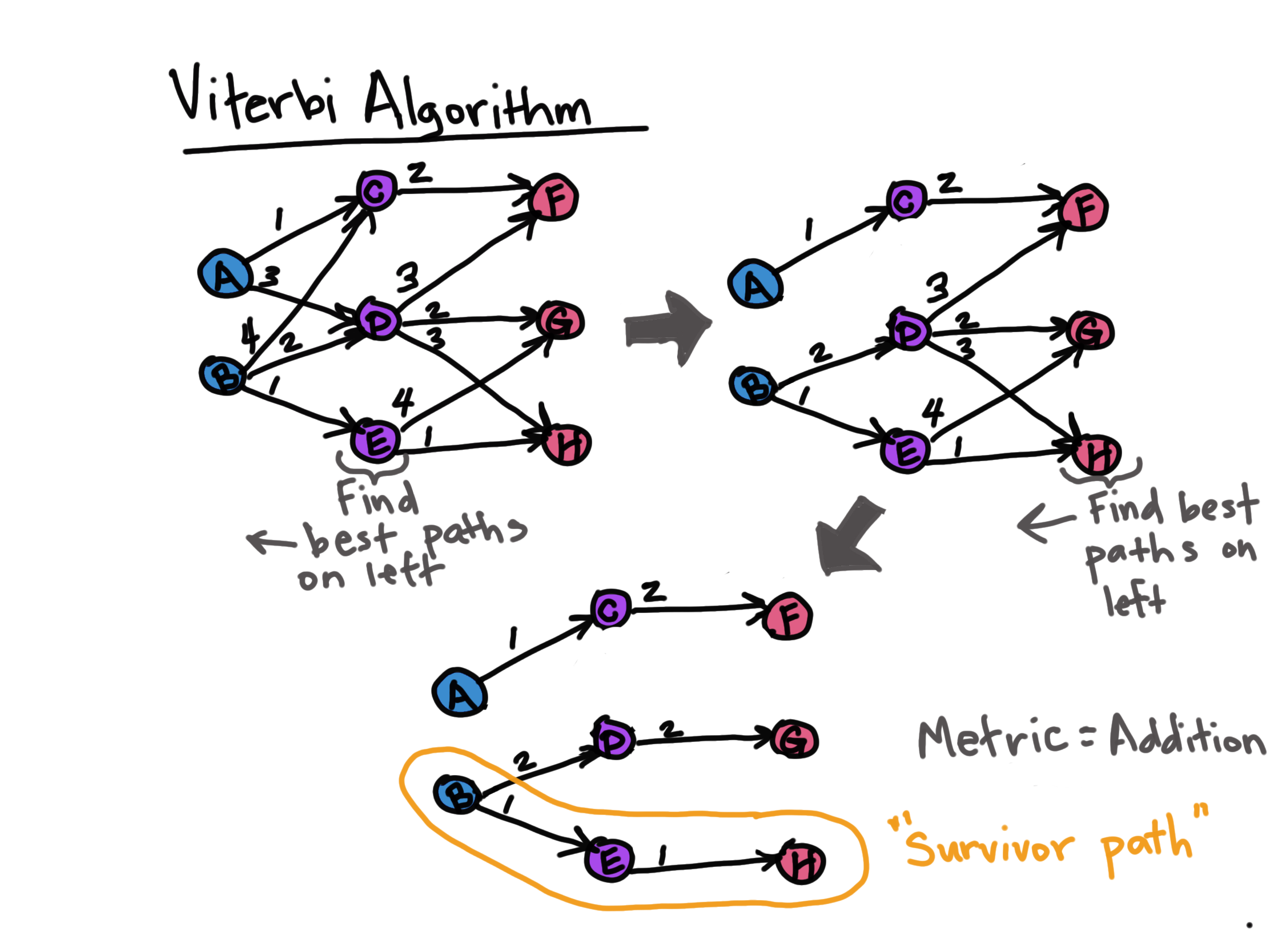
Viterbi Algorithm
If each Bi-LSTM instance (time step) has an associated output feature map and CRF transition and emission values, then each of these time step outputs will need to be decoded into a path through potential tags and a final score determined. This is the purpose of the Viterbi algorithm, here, which is commonly used in conjunction with CRFs.
Specifically, the Viterbi algorithm finds the optimal path through a sequence given a cost function by tracing backwards through a graph of all possible paths. There are computational tricks to finding this path in the high dimensional space and you can find out more in the PyTorch tutorial code link below (_forward_backwards_trick).
Here, let's see a simple example of just the Viterbi algorithm. The simplicity of Viterbi is that at each time step, it "looks to the left" to find that best path and then moves to the right, repeating this "look to the left" until a "survivor path" or optimal path is found with the last column being the possible tags. The score may also be found by tracing backwards along this path and using the metric decided upon.
In this example the optimal score (via a metric) is the lowest one, however, one could also look for the highest scoring path if another metric is used as is shown next.
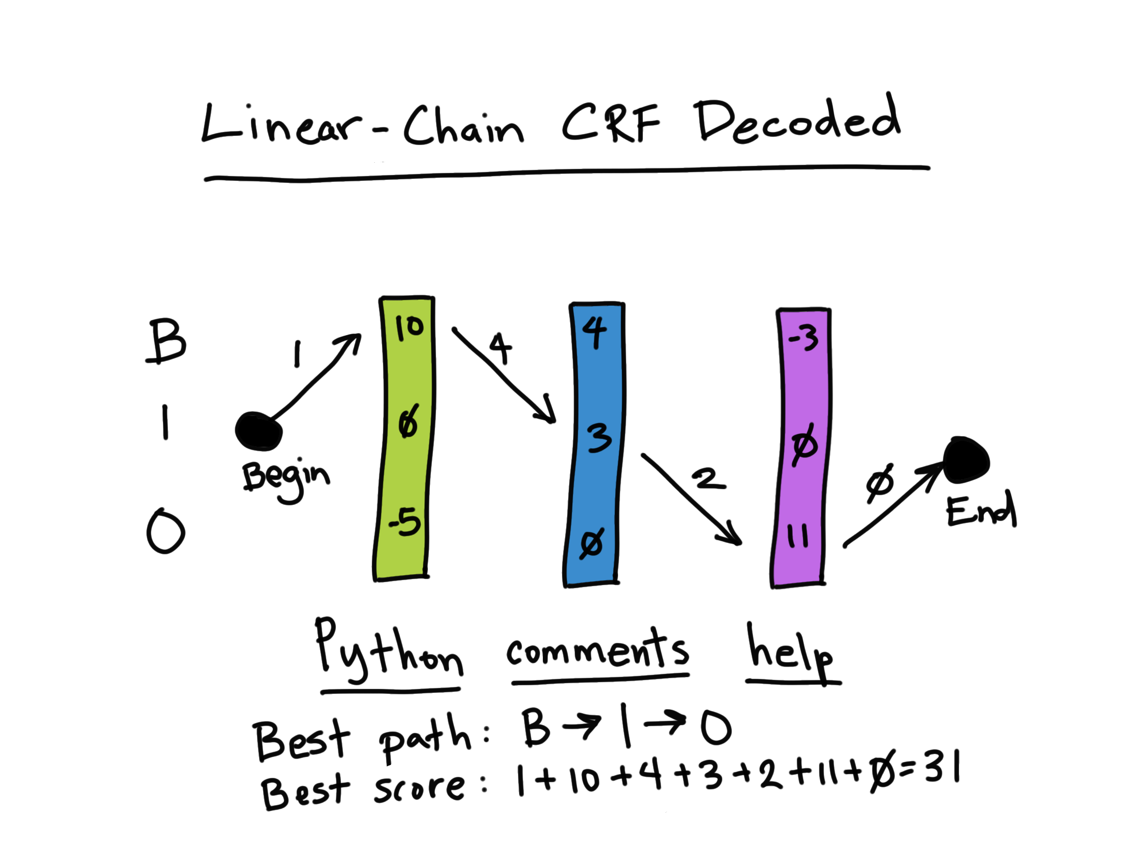
Getting more realistic...
With regards to our NER work here, below is an example of a "survivor" path within the context of the linear-CRF where we are trying to find the highest scoring path through a sequence (giving us the tags and final score). The transition matrix values are represented by the arrows and a sequence vector is shown as part of the overall cost function.
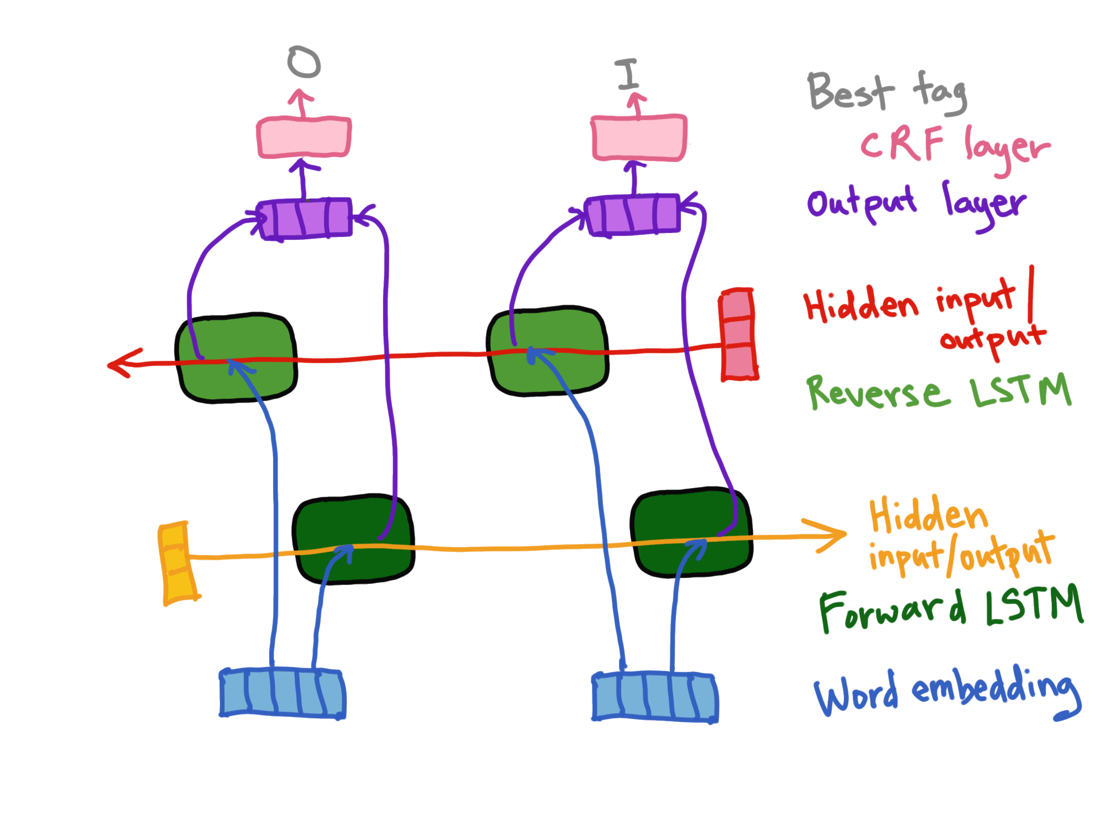
Putting it All Together
Here we have word embeddings as the data for the forward and reverse LSTMs. The resulting forward vector (V_f) and backwards vector (V_b or Output layer, here) are concatenated into a final vector (V_o) that feeds into the CRF layer and is decoded via the Viterbi algorithm (part of CRF layer) into the optimal tag for that input. Note, the initial values for the Hidden inputs for each LSTM (forward and reverse) are often a vector of random numbers.
For a more in-depth discussion, see this excellent post describing the Bi-LSTM, CRF and usage of the Viterbi Algorithm (among other NER concepts and equations): Reference.
Code
See this PyTorch official Tutorial Link for the code and good explanations.