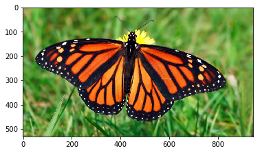
A Monarch butterfly courtesy of National Geographic Kids

tl:dr: Masks are areas of interest in an image set to one color, or pixel value, surrounded by a contrast color or colors. In this technical how-to, I use the OpenCV Python binding and Shapely library to create a mask, convert it to shapes as polygons, and then back to a masked image - noting some interesting properties of OpenCV and useful tricks with these libraries.
Posted: 2017-09-28
All of the code below can be found in this Python jupyter notebook.
Why are masks and polygons important? Imagine you'd like to identify all of the pixels in a brain scan that correspond to a certain feature of the brain - maybe identify the location and contours of a mass. Creating a mask, or highlighting just the feature's pixels on a backdrop of one contrast color, would be a good start, then understanding the shape of that masked feature as identified as polygons would give more information and perhaps help a doctor better understand any abnormalities. But say we had a machine that only identified shapes and we wanted the masked image. We could do so with the following process and code. Finally, and this is how I began exploring this topic, if one wanted to create a trained machine learning model for semantic image segmentation, or essentially classifying groups of pixels, a masked image and its class label (is this greenery or human-made structure?) plus shapes would be very nice to have for training.
My end goal was to turn a masked image (image with pixels of interest set to zero) into some polygon shapes and then back again using a couple of popular tools in Python. This was motivated by a real customer engagement around semantic image segmentation and I thought it might be useful to someone in the future.
Lesson 1:
opencvreads in as BGR andmatplotlibreads in a RGB, just in case that is ever an issue.
I tested this as follows:
img_file = 'monarch.jpg'

# Matplotlib reads as RGB
img_plt = plt.imread(img_file)
plt.imshow(img_plt)

# Read as unchanged so that the transparency is not ignored as it would normally be by default
# Reads as BGR
img_cv2 = cv2.imread(img_file, cv2.IMREAD_UNCHANGED)
plt.imshow(img_cv2)

# Convert opencv BGR back to RGB
# See https://www.scivision.co/numpy-image-bgr-to-rgb/ for more conversions
rgb = img_cv2[...,::-1]
plt.imshow(rgb)
With the following results:
Matplotlib RGB:

OpenCV BGR:
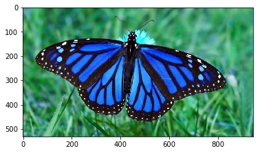
OpenCV BGR converted back:
Let's define our helper functions and not worry too much about the details right now (the original source of these helpers was a Kaggle post by Konstantin Lopuhin here - you'll need to be logged into Kaggle to see it).
Helper to create MultiPolygons from a masked image as numpy array:
def mask_to_polygons(mask, epsilon=10., min_area=10.):
    """Convert a mask ndarray (binarized image) to Multipolygons"""
    # first, find contours with cv2: it's much faster than shapely
    image, contours, hierarchy = cv2.findContours(mask,
                                  cv2.RETR_CCOMP,
                                  cv2.CHAIN_APPROX_NONE)
    if not contours:
        return MultiPolygon()
    # now messy stuff to associate parent and child contours
    cnt_children = defaultdict(list)
    child_contours = set()
    assert hierarchy.shape[0] == 1
    # http://docs.opencv.org/3.1.0/d9/d8b/tutorial_py_contours_hierarchy.html
    for idx, (_, _, _, parent_idx) in enumerate(hierarchy[0]):
        if parent_idx != -1:
            child_contours.add(idx)
            cnt_children[parent_idx].append(contours[idx])
    # create actual polygons filtering by area (removes artifacts)
    all_polygons = []
    for idx, cnt in enumerate(contours):
        if idx not in child_contours and cv2.contourArea(cnt) >= min_area:
            assert cnt.shape[1] == 1
            poly = Polygon(
                shell=cnt[:, 0, :],
                holes=[c[:, 0, :] for c in cnt_children.get(idx, [])
                       if cv2.contourArea(c) >= min_area])
            all_polygons.append(poly)
    all_polygons = MultiPolygon(all_polygons)

    return all_polygons
Helper to create masked image as numpy array from MultiPolygons:
def mask_for_polygons(polygons, im_size):
    """Convert a polygon or multipolygon list back to
       an image mask ndarray"""
    img_mask = np.zeros(im_size, np.uint8)
    if not polygons:
        return img_mask
    # function to round and convert to int
    int_coords = lambda x: np.array(x).round().astype(np.int32)
    exteriors = [int_coords(poly.exterior.coords) for poly in polygons]
    interiors = [int_coords(pi.coords) for poly in polygons
                 for pi in poly.interiors]
    cv2.fillPoly(img_mask, exteriors, 1)
    cv2.fillPoly(img_mask, interiors, 0)
    return img_mask
Lesson 2: If you want a more "blocky" polygon representation to save space or memory use the approximation method (add to the
mask_to_polygonsmethod).
    # Approximate contours for a smaller polygon array to save on memory
    contours = [cv2.approxPolyDP(cnt, epsilon, True)
                       for cnt in contours]
We read the image in again:
# Read in image unchanged
img = cv2.imread(img_file, cv2.IMREAD_UNCHANGED)

# View
plt.imshow(img, cmap='gray', interpolation='bicubic')
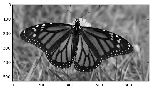
We convert to a luminance image with Scikit-Image's rgb2gray flattening it in the channel dimension:
# Convert to a luminance image or an array which is the same size as
# the input array, but with the channel dimension removed - flattened
BW = rgb2gray(img)

# View
plt.imshow(BW, cmap='gray', interpolation='bicubic')
With this result:
Lesson 3: For a quick mask we can use OpenCV's
convertScaleAbsfunction and it also is needed for the helper
As far as this pre-processing step goes, cv2.convertScaleAbs converts the image to an 8-bit unsigned integer with 1 channel, essentially flattening it and getting it ready to create some polygons (actually MultiPolygons in this case).
# Convert to CV_8UC1 for creating polygons with shapely
# CV_8UC1 is an 8-bit unsigned integer with 1 channel
BW = cv2.convertScaleAbs(BW)

# View
plt.imshow(BW, cmap='gray', interpolation='bicubic')
With this result:
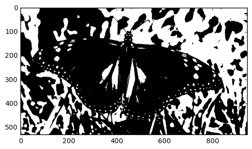
Now let's let our functions do the real work! Convert to polygons and then back to a masked image:
# Get the polygons using shapely
polys = mask_to_polygons(BW, min_area=50)

# Convert the polygons back to a mask image to validate that all went well
mask = mask_for_polygons(polys, BW.shape[:2])

# View - you'll see some loss in detail compared to the before-polygon
# image if min_area is high - go ahead and try different numbers!
plt.imshow(mask, cmap='gray', interpolation='nearest')
Final result:
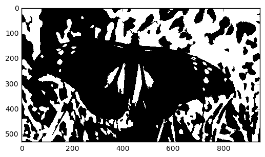
Notice the slight loss of detail - this is because we are removing really tiny polygons (see min_area parameter).
I leave it up to you to download this Python jupyter notebook and try using the RGB image for masking and creating Polygons and back. Do the results change? Try this on your own images and have fun!